Statistics
Imagine you work for a company that makes ball bearings. Your job is to make sure the ball bearings are the correct size. If you measured the diameter of ten ball bearings that were meant to be the same it is likely that you would find a range of values around an average.
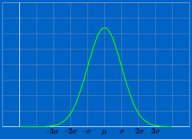
If you measured the diameters of a thousand ball bearings and plotted the diameters on a graph you would probably get a bell shaped curve. The width of the curve tells you how close the ball bearings are to the average diameter. A process that is well controlled will produce a narrow curve. A process that is poorly controlled will produce a wide curve.
The Mean
Two metrics that help us compare curves of this type are the mean and the standard deviation. The mean is the average value. Using the ball bearing example from the introduction, we find the mean by adding all the diameters together and then divide by the number of ball bearings.
If we measure all the ball bearings, the entire population, then we would use the symbols $\mu$ to represent the mean. If we measured a sample we would use the symbols $\bar{x}$ for the mean.
Population: $\mu=\frac{1}{N} \sum\limits_{i=1}^{N} x_i$
Sample: $\bar{x} = \frac{1}{N} \sum\limits_{i=1}^{N} x_i$
The Standard Deviation
The standard deviation is a measure of how far the values spread from the mean. The smaller the value for the standard deviation the better the process. If you measure the entire population you would use the symbol $\sigma$ to represent the standard deviation. If you measure a sample you would use the letter $s$ to represent the standard deviation.
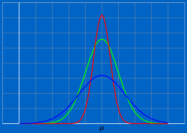
The red curve represents the best process with most of the values lying close to the mean. The green curve is not as good as the red curve. The Blue curve is the worst process with many values a long way from the mean.
$\mu$ is the population mean and $\sigma$ is the population deviation
$\bar{x}$ is the sample mean and $s$ is the sample deviation
If the population is normally distributed then, to a first approximation, 34% of the population lie between $\mu$ and $\mu + \sigma$. 14% lie between $\mu + \sigma$ and $\mu + 2\sigma$ and 2% lie between $\mu + 2\sigma$ and $\mu + 3\sigma$. This is a simplification but it is good enough for the moment.
| Interval | $-3\sigma$ | $-2\sigma$ | $-\sigma$ | $+\sigma$ | $+2\sigma$ | $+3\sigma$ |
| Percentage | 2% | 14% | 34% | 34% | 14% | 2% |
Calculating the Mean and Standard Deviation
If you measure an entire population the mean is given by
$\mu=\frac{1}{N} \sum\limits_{i=1}^{N} x_i$
and the standard deviation is given by
$\sigma = \sqrt{\frac{1}{N}\sum\limits_{i=1}^{N}(x_i-\mu)^2}$.
Population
$\mu=\frac{1}{N} \sum\limits_{i=1}^{N} x_i$
$\sigma = \sqrt{\frac{1}{N}\sum\limits_{i=1}^{N}(x_i-\mu)^2}$
If you take $N$ samples from a population like a production line the mean is given by
$\bar{x} = \frac{1}{N} \sum\limits_{i=1}^{N} x_i$
and the standard deviation is given by $s=\sqrt{\frac{1}{N-1}\sum\limits_{i=1}^{N}(x_i-\bar{x})^2}$
Sample
$\bar{x} = \frac{1}{N} \sum\limits_{i=1}^{N} x_i$
$s=\sqrt{\frac{1}{N-1}\sum\limits_{i=1}^{N}(x_i-\bar{x})^2}$
Confidence Interval
If we measure a characteristic of an entire population we can trust our values for $\mu$ and $\sigma$ (assuming our measurements are valid). If we measure the same characteristic of a sample we have to treat our values for $\bar{x}$ and $s$ with care because, in general terms, they will not be the same as $\mu$ and $\sigma$ for the population.
In the introduction we discussed ball bearing with a nominal diameter of $10$mm. If we chose a ball at random we could be 100% confident that the diameter would lie between $0$mm and $20$mm, we could be reasonably confident that the diameter would lie between $9$mm and $11$mm. How confident could we be that the diameter lies between $9.95$mm and $10.05$mm?
To find out we calculate a confidence interval, that is, a lower and upper value for which we have a predetermined confidence. The confidence interval is defined to be $\bar{x} \pm z \frac{s}{\sqrt{n}}$ where $\bar{x}$ is the sample mean, $z$ is the confidence factor, $s$ is the sample deviation and $n$ is the number of samples.
Confidence interval = $\bar{x} \pm z \frac{s}{\sqrt{n}}$
where $\bar{x}$ is the sample mean, $z$ is the confidence factor, $s$ is the sample deviation and $n$ is the number of samples
The confidence factor is calculated to be 1.282 for 80% confidence up to 3.291 for 99.9% confidence, see below
| Confidence | 80% | 85% | 90% | 95% | 99% | 99.9% |
| Factor $z$ | 1.282 | 1.440 | 1.645 | 1.960 | 2.576 | 3.291 |