Regression
When you analyse experimental data you will want to see whether there is any relation between the sets of data. One way to do this is to calculate the Pearson product-moment correlation coefficient.
Pearson's Product-Moment Correlation Coefficient
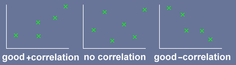
Karl Pearson devised a coefficient to measure the correlation between two sets of data. The coefficient ranges from $-1$ to $1$. A value of $1$ means there is perfect correlation between the data sets, a value of $0$ means there is no correlation and a value of $-1$ means there is perfect negative correlation between the data sets. Note: independent data may be strongly correlated, correlation does not mean causality.
Assume you have a set of independent data $x$ with corresponding dependent data $y$ then Pearson's product-moment correlation coefficient is given by:
$r=\dfrac{n \sum xy- \sum x \sum y}{\sqrt{n\sum x^2-(\sum x)^2} \times \sqrt{n\sum y^2-(\sum y)^2}}$
where $n$ is the number of samples and $\sum$ means the sum of the values in the set of data
If the value of $|r| \lt 0.5$ then the correlation is weak or non-existent. If the value of $|r| \geq 0.5$ then there is a correlation between the two sets of data.
If $|r| \geq 0.5$ then you will want to find the gradient and y-intercept of the regression line. To do this we will use the method of least squares. Least squares minimises the square of the perpendicular distance between each data point and the regression line. The square of the distance is used because points below the line give a negative distance and we want to minimise to sum of all the separate distances. The gradient and y-intercept are given by:
$m = \dfrac{n \sum xy- \sum x \sum y}{n\sum x^2-(\sum x)^2}$
$c = \dfrac{\sum x^2 \sum y- \sum x \sum xy}{n\sum x^2-(\sum x)^2}$
Example 1: Given the following data calculate the Pearson correlation coefficient.
| $x$ | 0 | 1 | 2 | 3 | 4 |
| $y$ | 8 | 14 | 13 | 20 | 19 |
To find $r$ we need $\sum x$, $\sum y$, $\sum xy$, $\sum x^2$, $\sum y^2$ and $n$.
| $x$ | 0 | 1 | 2 | 3 | 4 | 10 |
| $y$ | 8 | 14 | 13 | 20 | 19 | 74 |
| $xy$ | 0 | 14 | 26 | 60 | 76 | 176 |
| $x^2$ | 0 | 1 | 4 | 9 | 16 | 30 |
| $y^2$ | 64 | 196 | 169 | 400 | 361 | 1190 |
Putting these values into Pearson's equation
$r=\dfrac{n \sum xy- \sum x \sum y}{\sqrt{n\sum x^2-(\sum x)^2} \times \sqrt{n\sum y^2-(\sum y)^2}}$
$=\dfrac{5 \times 176 - 10 \times 74}{\sqrt{5 \times 30 - 10^2} \times \sqrt{5 \times 1190 - 74^2}}$
$=0.909$
A value for $r=0.909$ means there is a high correlation for these data which means it is worth calculating the gradient and y-intercept of the correlation line.
$m=\dfrac{n \sum xy- \sum x \sum y}{n\sum x^2-(\sum x)^2}$
$=\dfrac{5 \times 176 - 10 \times 74}{5 \times 30 - 10^2}$
$=2.80$
$c=\dfrac{ \sum x^2 \times \sum y - \sum x \sum xy}{n\sum x^2-(\sum x)^2} $
$=\dfrac{30 \times 74 - 10 \times 176}{5 \times 30 - 10^2}$
$=9.2$
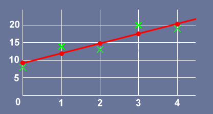
Here is a plot of the data and the regression line
Non-linear Regression
In this section we will consider problems where some function of the dependent variable can be used in place of the variable itself. As an example consider a simple pendulum. The period of a simple pendulum is given by $t = 2 \pi \sqrt{\dfrac{l}{g}}$. If we plot $t$ for a range of values of $l$ we get a quadratic curve. If, on the other hand, we plot $t^2$ for a range of values of $l$ we get a straight line and that simplifies the arithmetic.
Altitude (km) Time (s) Time2 (s2 x1000)
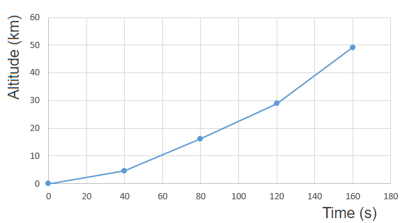
Example 2: The following data is the altitude (km) of a rocket at given times (s) after launch.
| Time (s) | 0 | 40 | 80 | 120 | 160 |
| Altitude (km) | 0 | 4.7 | 16.2 | 28.9 | 49.1 |
Here is a plot of the data.
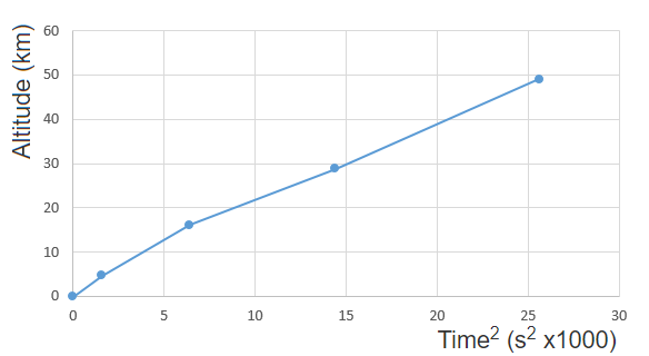
We know the curve is of the form $\dfrac{1}{2}at^2$ so instead of plotting altitude vs time we will plot altitude vs time2. Here is a plot.
To find Pearsons correlation coefficient $r$ we need $\sum x$, $\sum y$, $\sum xy$, $\sum x^2$, $\sum y^2$ and $n$.
| $x$ | 0 | 1600 | 6400 | 14400 | 25600 | 48 |
| $y$ | 0 | 4700 | 16200 | 28900 | 49100 | 98900 |
| $xy$ | 0 | 7.52 | 103.7 | 416.2 | 1257 | 1784 |
| $x^2$ | 0 | 2.56 | 40.96 | 207.4 | 655.4 | 906.2 |
| $y^2$ | 0 | 22 | 262 | 835 | 2411 | 3530 |
Putting these values into Pearson's equation
$r=\dfrac{n \sum xy- \sum x \sum y}{\sqrt{n\sum x^2-(\sum x)^2} \times \sqrt{n\sum y^2-(\sum y)^2}}$
$=\dfrac{5 \times 1784 - 48 \times 98.9}{\sqrt{5 \times 906.2 - 48^2} \times \sqrt{5 \times 3530 - 98.9^2}}$
$=0.9970$
A value for $r=0.9970$ means there is a high correlation for these data which means it is worth calculating the gradient.
$m=\dfrac{n \sum xy- \sum x \sum y}{n\sum x^2-(\sum x)^2}$
$=\dfrac{5 \times 1784 - 48 \times 98.9}{5 \times 906.2 - 48^2}$
$=1.87$
Remember $s=\dfrac{1}{2}at^2$. We have plotted $s$ against $t^2$ so the gradient $=\dfrac{1}{2}a$ and the acceleration is $3.75$ m/s2.